Constructing Efficient Simulated Moments Using Temporal Convolutional Networks
Jonathan Chassot and Michael Creel
Deep Learning for Solving and Estimating Dynamic Models
(DSE2023CH)
August 24, 2023
Our Contribution
- Propose a method to estimate model parameters leveraging
deep learning - Allow for inference using
well-established econometric methods - Provide an
exactly identifying andinformative set of statistics for simulation-based inference - Achieve performance equal to or better than maximum likelihood for small and moderate sample sizes for several DGPs
Motivating Example
- Parameter estimation for a complex data-generating process (DGP)
- Failure of traditional estimation methods (ML, GMM)
Motivating Example
- Parameter estimation for a complex data-generating process (DGP)
- Presence of latent variables
- High-dimensional integrals
- …
- Failure of traditional estimation methods (ML, GMM)
- Intractable likelihood
- Computational constraints
- No closed-form theoretical moments
Methodology
Simulation-based Inference
- Method of Simulated Moments (McFadden, 1989)
- Approximate Bayesian Computation (Rubin, 1984)
- Indirect Inference (Gouriéroux, Monfort & Renault, 1993; Smith, 1993)
- Bayesian Limited Information Estimation (Kwan, 1999; Kim, 2002; Chernozhukov & Hong, 2003)
Method of Simulated Moments
- Use
simulated moment conditions instead of theoretical ones - Match data moments and simulated moments
$$
\hat{\theta}_{\text{MSM}} = \underset{\theta \in \Theta}{\arg \min} \ \left(T^{-1}\sum_{t=1}^T m(x_t, \theta)^{\top}\right) W_T \left(T^{-1}\sum_{t=1}^T m(x_t, \theta)\right),
$$
where $W_T$ is a weighting matrix and
$$m(x_t, \theta) = f(x_t) - \frac{1}{S} \sum_{s=1}^S f(\tilde{x}_t(\theta))$$
with $S$ the number of simulations and $\tilde{x}_t(\theta)$ the data simulated at parameter $\theta$.
Method of Simulated Moments
- …but how do we choose $f(\cdot)$ in
$$m(x_t, \theta) = f(x_t) - \frac{1}{S} \sum_{s=1}^S f(\tilde{x}_t(\theta))$$
Optimal Moment Conditions
- Choosing optimal moment conditions is difficult
- Overidentification leads to high asymptotic efficiency but also to
high bias and/or variance in finite samples (Donald, Imbens & Newey, 2009)
Optimal Moment Conditions
- Choosing optimal moment conditions is difficult
- Overidentification leads to high asymptotic efficiency but also to
high bias and/or variance in finite samples (Donald, Imbens & Newey, 2009)
Theory:
- Gallant & Tauchen (1996) show that the optimal choice of moment conditions corresponds to the
score function (equivalent to MLE)
Practice:
- Moment selection criteria and algorithms (e.g., Donald, Imbens & Newey, 2009; Cheng & Liao, 2015; DiTraglia, 2016)
- Our work is related to this category
Optimal Moment Conditions
Goal:
- Given a data set $\{x_t \mid x_t \in \mathbb{R}^k\}_{t=1}^T$, generated by our DGP under true parameter value $\theta_0$, we would like to find $f(x_t) \approx \theta_0$
Optimal Moment Conditions
Goal:
- Given a data set $\{x_t \mid x_t \in \mathbb{R}^k\}_{t=1}^T$, generated by our DGP under true parameter value $\theta_0$, we would like to find $f(x_t) \approx \theta_0$
Idea:
- Generate samples $\{\tilde{x}_t(\theta) \mid \tilde{x}_t(\theta) \in \mathbb{R}^k\}$ with $\theta \in \Theta$ and use deep learning to infer $f(\cdot)$, a
mapping from data to parameters
Neural Networks
- Long Short-Term Memory Networks (LSTM)
- Temporal Convolutional Networks (TCN)
Neural Networks
- Long Short-Term Memory Networks (LSTM)
- Hochreiter & Schmidhuber (1997)
- Dominated sequence modelling pre-Transformers (Vaswani et al., 2017)
- Difficulties in modeling long-term dependencies
- Serve as a
baseline deep learning model in this work - Temporal Convolutional Networks (TCN)
- Introduced as WaveNet (van den Oord et al., 2016)
- Fully parallelizable
- Flexible receptive field size
- Serve as the
main model in this work
Benchmark Results
Results for Simple DGPs
- Benchmark our TCNs and LSTMs against MLE for 3 data-generating processes (MA(2), Logit, GARCH(1,1)) where the
likelihood is tractable - Sample sizes 100, 200, 400, and 800
- Comparison across 5'000 test samples for each setting
Conjecture: if the neural networks do well, they will also perform well when the MLE is not available


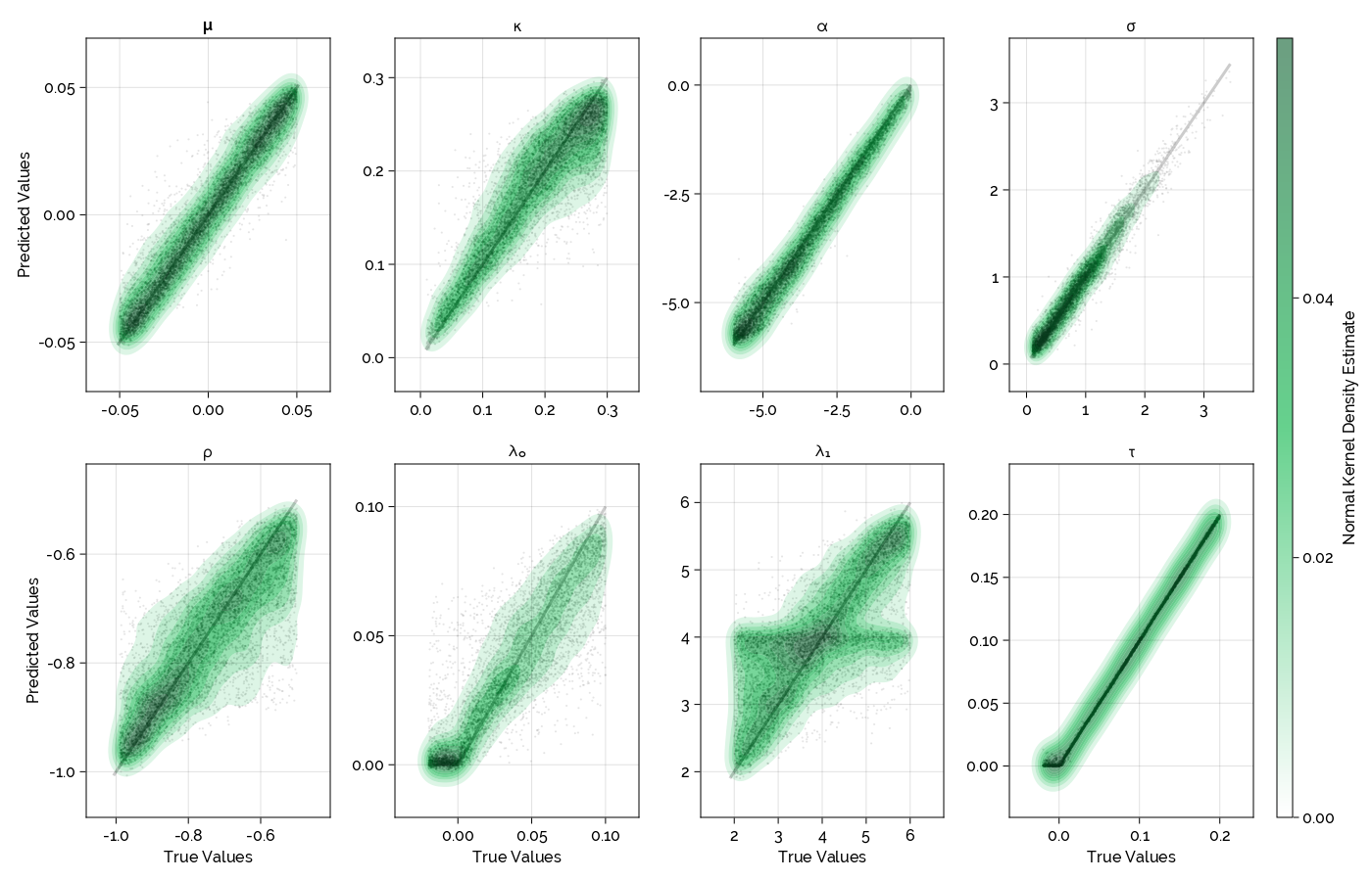
Jump-Diffusion Process
Jump-Diffusion Stochastic Volatility
$$
\begin{align*}
dp_{t} & =\mu \, dt+\sqrt{\exp h_{t}} \, dW_{1t}+J_{t} \, dN_{t}\\
dh_{t} & =\kappa(\alpha-h_{t})+\sigma \, dW_{2t}
\end{align*}
$$
Jump-Diffusion Stochastic Volatility
$$
\begin{align*}
dp_{t} & =\mu \, dt+\sqrt{\exp h_{t}} \, dW_{1t}+J_{t} \, dN_{t}\\
dh_{t} & =\kappa(\alpha-h_{t})+\sigma \, dW_{2t}
\end{align*}
$$
- $p_t$: logarithmic price
- $\mu$: average drift in price
- $J_t$: jump size ($J_t = a \lambda_1 \sqrt{\exp h_t}$) with $\mathbb{P}[a=1]=\mathbb{P}[a=-1]=\frac{1}{2}$
- $N_t$: Poisson process with jump intensity $\lambda_0$
- $h_t$: logarithmic volatility
- $\kappa$: speed of mean-reversion
- $\alpha$: long-term mean volatility
- $\sigma$: volatility of the volatility
- $W_{1t}, W_{2t}$: correlated Brownian motions with correlation $\rho$
Jump-Diffusion Stochastic Volatility
- $\mu$: average drift in price
- $\kappa$: speed of mean-reversion
- $\alpha$: long-term mean volatility
- $\sigma$: volatility of the volatility
- $\rho$: correlation between $W_{1t}$ and $W_{2t}$
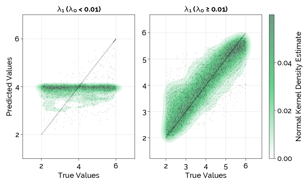
- $\lambda_0$: jump intensity
- $\lambda_1$: jump magnitude
- $\tau$: the volatility of a measurement error $N(0, \tau^2)$ added to the observed price
- logarithmic returns
- realized volatility
- bipower variation
Conclusion
Conclusion
- Best case scenario for deep learning
- Once the network is trained, inference is as fast as matrix multiplication
- Limited only in the cost of simulation
- Promising results on three simple DGPs and one moderately complex DGP
- Easy to implement
- Full Julia package under development (already functional):
https://github.com/JLDC/DeepSimulatedMoments.jl