A Simple Recurrent Model in Flux

After spending some time in the Julia discourse forum, I noticed that there are some difficulties in understanding how one should implement recurrent neural networks in Flux.

In this post, I will briefly go over the necessary steps to implement a straightforward recurrent model in Flux. This post proposes a purely applied approach; I will not be discussing the theory behind recurrent models. I also highly recommend reading the Flux documentation on recurrent models, as it contains a lot more information than this post.

This post aims to provide a 5-minute guide on how to implement the most basic recurrent model in Flux. It skips many details, crucial to building efficient recurrent models, but it should be sufficient to get you started. Future blog posts will go into more detail on how to set up good recurrent models.

Sequence-to-sequence modeling on univariate data

Let’s admit that we are interested in a sequence-to-sequence modeling task on a univariate time series. That is, we have some time-series data $\{x_t : t = 1, \dots, T\}$ and at each time step $t$, we wish to predict the value of $x_{t+1}$.

For instance, we might want to try and predict a stock’s closing price for the following day; this is an arduous task, and doing well will realistically require more than running a basic recurrent model on the past prices. Nevertheless, it is a simple, attractive example that we can use to explain the foundations of recurrent modeling in Flux.

Data

First, we need some data. I will try to make another blog post at some point on different ways to obtain data directly using Julia. However, we will assume that we already have the data for the time being. We will use stock data for Apple Inc. (AAPL) between the start of 2019 and the end of 2021; you can download the data in CSV format from my site.

# Load necessary packages to read CSV data
using CSV, DataFrames 
# Load the AAPL data into a DataFrame
data = CSV.read("AAPL.csv", DataFrame)
# Keep only the close price, and convert the datatype to Float32, 
# Float32 is NECESSARY for recurrent models in Flux
price = Float32.(data.Close)
# Create a vector of features (our input) and a vector of labels (our target output)
X = price[1:end-1]
Y = price[2:end]

Let’s take a step back and recapitulate. We have a time series of close prices for the AAPL stock. We have a vector X and a vector Y, with a length of 756. Y is simply the vector of prices shifted by one day, i.e., Y[t] is tomorrow’s closing price.

Recurrent data in Flux

The first tricky thing is that we need to convert the data into a format Flux can understand. Flux expects a different data shape than most other machine learning libraries such as PyTorch or TensorFlow.

Typically, recurrent models expect input data in the form of 3-dimensional arrays with structure (features sequence_length, batch_size). Flux expects a vector of length sequence_length with structure (features, batch_size).

To keep things simple, we will work with the entire sequence length of 756. Furthermore, we have a single feature (today’s closing price) and a single batch. In other words, we can reshape the input data as follows:

# Reshape input data into Flux recurrent data format
X = [[x] for x ∈ X]

If our input data were multivariate or had multiple batches, we would have to reshape our data differently. I will cover this in a future post. In the meantime, if this is what you are looking for, look at this file, specifically the functions tabular2rnn and rnn2tabular.

Recurrent model

There are a lot of details I omitted, such as choosing a sensible sequence length, normalizing the data, and so on. While these are not relevant to our example, they are crucial to building a good deep learning model.

Creating a recurrent neural network model in Flux is as easy as possible, and the code is self-explanatory.

using Flux # Load Flux
# Create a model with an RNN layer and a fully-connected layer
model = Chain(
    RNN(1 => 32, relu),
    Dense(32 => 1, identity)
)

That’s it, model is a neural network composed of 2 chained layers, a recurrent layer with input dimension 1, output dimension 32, and ReLU activation, and a fully-connected layer with input dimension 32, output dimension 1, and linear activation.

Training the model

Now we are ready to train our model. We will train our model for 100 epochs using the Adam optimizer and the mean squared error loss.

Note that Flux comes with a multitude of optimizers and loss functions, but it is also possible (and relatively easy) to define your own.

# Train the model
epochs = 100
opt = ADAM()
θ = Flux.params(model) # Keep track of the model parameters
for epoch ∈ 1:epochs # Training loop
    Flux.reset!(model) # Reset the hidden state of the RNN
    # Compute the gradient of the mean squared error loss
    ∇ = gradient(θ) do
        model(X[1]) # Warm-up the model
        sum(Flux.Losses.mse.([model(x)[1] for x ∈ X[2:end]], Y[2:end]))
    end
    Flux.update!(opt, θ, ∇) # Update the parameters
end

That’s it. We have loaded data, created and trained a recurrent model in less than 35 lines of code… Julia and Flux are pretty impressive!

Visualizing the results

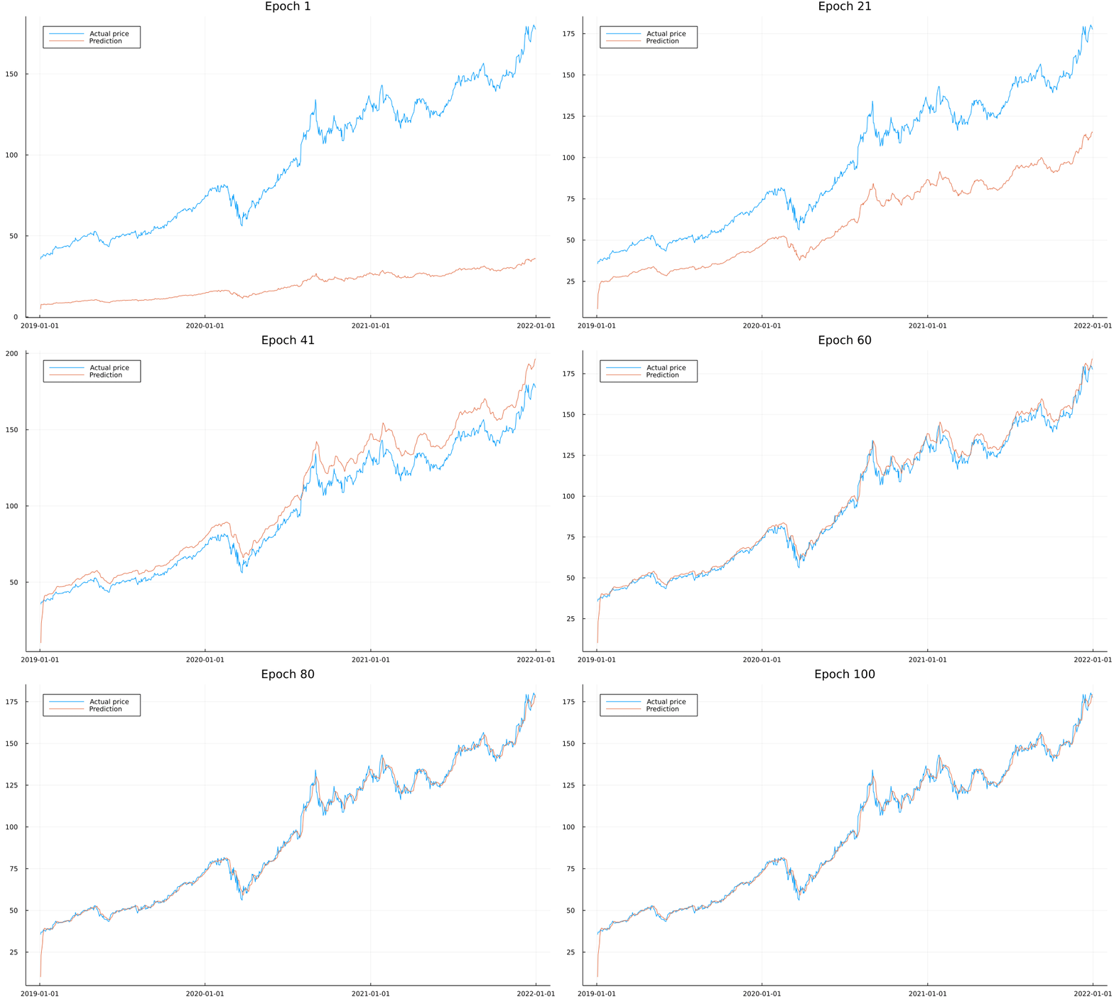
Finally, let’s have a glance at what the predictions look like to make sure our model works:

As we see, our model is doing what it should and converges after around 50 epochs. I won’t lie and claim you could use it to accurately predict stock prices as there are a lot of important details we haven’t yet covered, such as overfitting. We also see how the first prediction is far off; this is due to us never training the model on the first day of the data and only using it to warm up our internal model state.